
Welcome to the first entry in my new series: Research Papers Reviewed & Coded.
In the field of AI, it’s easy to become lost in the excitement surrounding the latest LLMs and frameworks. We import libraries like “Magic” and ignore the technology underlying. I feel that you can not completely grasp an algorithm until you can create it from scratch.
In this series, I am going back to the basics. I’ll be reading the foundational papers that founded the field of artificial intelligence, breaking down their math, and implementing their algorithms in raw Python no Keras or PyTorch, just the arithmetic.
We begin with the paper that ended the AI Winter and gave us the blueprint for Deep Learning.
Table of Contents
Executive Summary
- Paper: Learning Representations by Back-propagating Errors
- Authors: David Rumelhart, Geoffrey Hinton, and Ronald Williams
- Year: 1986
In the mid-1980s, Artificial Intelligence was experiencing a “Winter.” The optimism of the 1960s was beginning to fade as researchers encountered a stumbling block: early neural networks (such as the Perceptron) were unable to address nonlinear issues. They were said to have “all setup, no payoff.”
The publication of “Learning Representations by Back-propagating Errors” in 1986 changed the course of the field forever. Rumelhart, Hinton, and Williams did more than merely provide an algorithm; they also established a mathematical foundation for training hidden layers, allowing networks to create internal representations of complex data..
This review explores the 1986 article, delving into the mathematical physics of backpropagation, the specific limits it overcome (the Symmetry Problem), and its basic impact on modern Deep Learning systems.
1. The Challenge: The Limits of Linearity
To understand the breakthrough, we must first grasp the obstacle at hand. Prior to backpropagation, neural networks did not have any “hidden” layers. They mapped inputs to outputs.
The Linearity Trap
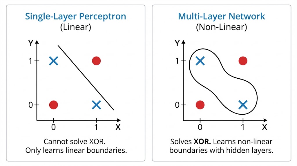
These networks were only able to tackle problems that were linearly separable. If you could draw a straight line through the data and classify it, the network worked. If the data seemed complicated or “tangled,” the network would fail.
The paper highlights the Symmetry Problem to illustrate this.
Imagine a network that receives a vector of binary inputs (e.g., [1, 0, 0, 1]). The goal is to detect if the pattern is symmetrical around its center.
- The Limitation: A typical perceptron examines inputs individually. A single input unit (such as the first 1) provides no evidence for or against symmetry on its own. Symmetry is a characteristic of the whole, not its component parts.
- The Analogy: According to the briefing, this restriction is “trying to understand a whole painting by just looking at one tiny brush stroke at a time.” Without the ability to merge these “brush strokes” into intermediate characteristics, the network is unable to see the entire image.
The “Hidden” Solution
Researchers hypothesized that placing intermediary layers between the input and output could fix this. These hidden units could function as feature detectors, recording combinations of inputs.
- The Hurdle: There was no instructor. In the output layer, we know the “correct” answer and can calculate the error. However, we have no idea what value a hidden unit in the center of the network should have had. How can you put blame to a neuron that is not directly related to the outcome?
2. The Algorithm: Backpropagation of Errors
The authors introduced a procedure to “assign blame” by propagating the error signal backward through the network.
The Mathematical Framework
The algorithm is an application of the Chain Rule from calculus to minimize the error function.
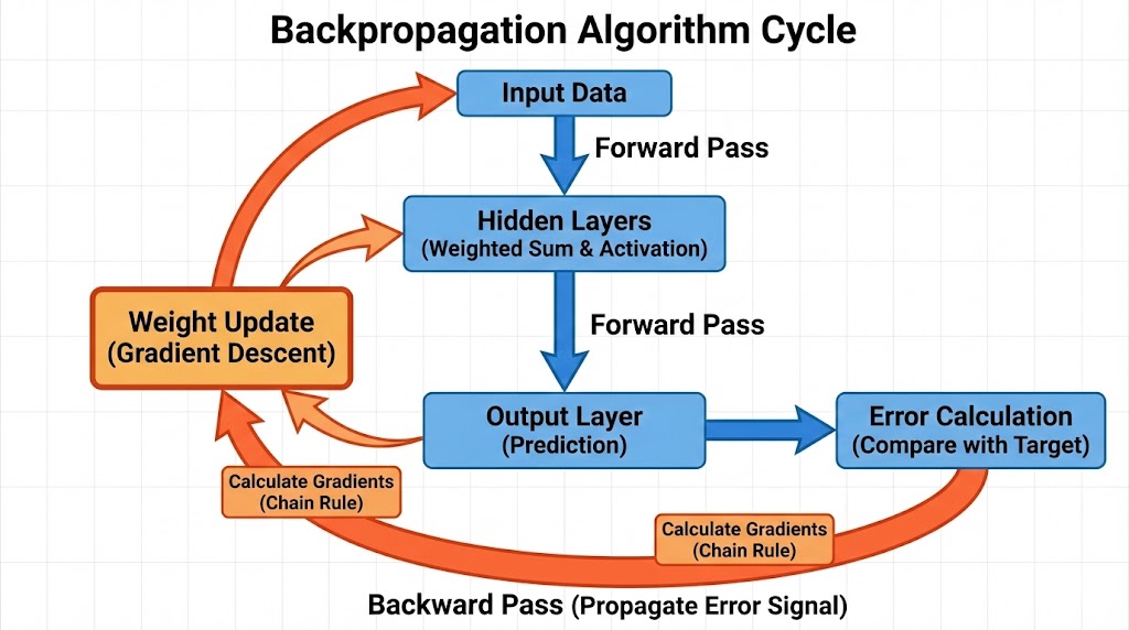
Step 1: The Forward Pass
The input passes through the network. For each unit j, the output yj is computed by running the weighted sum of its inputs through a non-linear activation function (the study used the logistic sigmoid):
Step 2: Error Calculation
The system calculates the Total Error (E) at the output layer. The paper defines this as the squared difference between the actual output (y) and the desired target (d):
(Where c iterates over input cases and j over output units).
Step 3: The Backward Pass (Gradient Calculation)
This is the central innovation. To change a weight, we must understand the partial derivative of the Error with regard to that weight (∂E/∂w). The algorithm uses the Chain Rule to compute the error signal (commonly represented as δ) for the output units, which is subsequently passed backward to the hidden units.
- The error signal for a hidden unit is the weighted sum of the error signals from the units it connects to in the next layer, multiplied by the derivative of its activation function.
The Weight Update: Gradient Descent with Momentum
Once the gradient is known, the weights are updated. However, the paper introduced a critical addition that is often overlooked in simple explanations: Momentum.
Standard Gradient Descent may fluctuate or become stuck in local minima. To address this issue, the authors changed the update rule to include a percentage of the previous weight change.
The update rule is:
εepsilon): The learning rate.∂E/∂w(t): The gradient (slope).- α (alpha): The Momentum term. This term effectively gives the weight updates “inertia,” helping the network plow through small local minima and converge faster.
3. Why Backprop? The Computational Advantage
The paper explicitly discusses why this method was chosen over other mathematical optimization techniques, such as Newtonian methods (second-derivative methods).
While Newtonian methods can theoretically find the minimum of an error surface faster (in fewer steps), they require calculating the Hessian matrix—a matrix of second derivatives.
- Computational Cost: Calculating the Hessian requires memory and operations on the order of
O(N2)whereN is the number of weights. - Backprop Efficiency: Backpropagation only calculates the first derivative (gradient), which scales linearly
O(N).
This was reasonable for 1986’s modest networks. For today’s huge networks (with billions of parameters), N2 is impossible. Backpropagation’s linear scaling is the main reason Deep Learning is computationally feasible today. Furthermore, the technique is extremely parallelizable, a trait that was dormant until the introduction of contemporary GPUs.
4. The “Family Tree” Experiment: Learning Representations
The most profound claim of the paper was that backpropagation allows networks to create their own “internal language.” To prove this, the authors devised the Family Tree Experiment.
The Setup
The network was trained on 104 triples representing family relationships in two isomorphic family trees (one English, one Italian).
- Input:
(Colin, has-father) - Target Output:
(James)
The Result
The network never received knowledge of the “nationality,” “generation,” or “branch of the family.” It simply recognized names and relationships. However, after training, the writers examined the weights of the hidden units and discovered something remarkable:
- Unit 1: Had learned to distinguish between the English family and the Italian family.
- Unit 2: Had learned to encode “generation” (classifying people as parents, children, or grandparents).
- Unit 3: Had learned to encode the specific branch of the family tree.
The abstract concepts that control the data were discovered naturally by the network. It was more than just memorization; it was also about understanding the framework. This demonstrated that hidden units function as sophisticated feature extractors.
5. Limitations and Critique
The authors were rigorous scientists and candidly acknowledged the limitations of their new procedure.
1. Local Minima
Gradient descent ensures finding a minimum, but not always the global (lowest possible) minimum. The error surface of a neural network resembles a large landscape of hills and valleys; the algorithm may become trapped in a small valley (local minimum) and miss the deeper valley nearby.
- Retrospective: While a major concern in 1986, modern research suggests that in high-dimensional spaces, local minima are rarely a showstopper for deep networks.
2. Biological Plausibility
Perhaps the most famous disclaimer in the paper is regarding the human brain. The authors admitted that backpropagation is “not a plausible model of learning in brains.”
There is no known mechanism in the biological brain that propagates error signals backward along axons in the way the algorithm describes. While the result (learning representations) mimics human capability, the mechanism is distinctly artificial.
6. Connecting Theory to the Modern Stack
The 1986 article may appear to be a history lesson, but for a Machine Learning Engineer, it is a manual for how your everyday tools function. If you use TensorFlow/Keras or PyTorch, you interact with the Rumelhart-Hinton-Williams method in almost every line of training code.
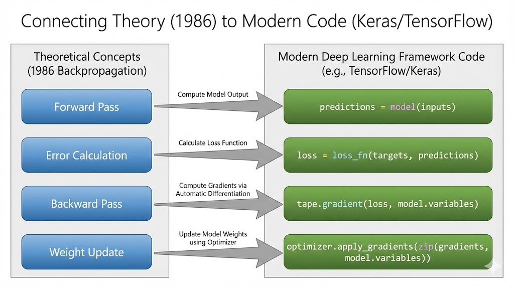
The libraries simply wrap the calculus in efficient C++ or CUDA operations. Here is the direct mapping between the paper’s concepts and the modern stack:
The Mapping
| The 1986 Concept | The Modern Code (Keras/TensorFlow) | What Is Happening Under the Hood? |
| Forward Pass | predictions = model(inputs) | The system computes the weighted sums and applies activation functions (like ReLU or Sigmoid) layer by layer. |
| Error Calculation | loss = loss_fn(targets, predictions) | This calculates the E (Total Error). While the study used Sum of Squared Errors (SSE), we frequently use Cross-Entropy nowadays, but the approach of calculating a scalar “loss” value is the same. |
| Backward Pass | tape.gradient(loss, model.variables) | This is the Backpropagation step. The framework creates a computational graph and walks it backward, using the Chain Rule to calculate ∂E/∂w for every parameter. |
| Momentum | optimizer = SGD(momentum=0.9) | The “alpha” concept used in the study is specifically defined here. Modern optimizers, such as Adam, extend this approach by tracking both momentum (first instant) and variance (second moment). |
| Weight Update | optimizer.apply_gradients(...) | This is the Gradient Descent step. It applies the update rule δw derived in the paper to shift weights downhill. |
| The Loop | model.fit() | This high-level function orchestrates the entire cycle of Forward ⇒ Backward ⇒ Update⇒ Repeat. |
Why This Matters for Debugging
Understanding this connection makes you a better engineer.
- Vanishing Gradients: If you realize that backpropagation is based on multiplying derivatives (Chain Rule), you can see why deep networks failed during the 1980s. Multiplying multiple little integers (such as the derivative of a sigmoid) produces a minor gradient near the input layers. This explains why we moved to ReLU (whose derivative is simply 1 or 0) to maintain signal strength.
- Learning Rate Explodes: If your loss turns to
NaN, you know from the update equationΔw=- ε (∂E/∂w)that your learning rate (ε) might be too high, causing the weights to jump too far and destabilize the error calculation.
It is worth mentioning that, while this 1986 algorithm was flawless, it took over 25 years for hardware (GPUs) and data volumes (the Internet) to catch up with the math, resulting in the Deep Learning revolution in the 2010s.
7. Code Implementation
Theory is useful, but code is proof.
To demonstrate that the 1986 algorithm works exactly as described, I built the entire technique from scratch. I purposefully avoided utilizing current frameworks such as TensorFlow and PyTorch. Instead, I used raw Python and NumPy to manually calculate the derivatives and apply the chain rule.
In this version, the network solves the XOR Problem, which early perceptrons were famously unable to solve.
You can view the full source code, including the manual implementation of the Momentum term and the Sigmoid derivative, in my GitHub repository:
View the Code on GitHub: Research Papers Reviewed & Coded
(Note: This repository will be updated as I review and implement more foundational papers in this series.)
8. Conclusion: The Seed of the AI Revolution
Reviewing “Learning Representations by Back-propagating Errors” nearly four decades later is a humbling experience. It reveals that the core engine driving today’s trillion-dollar AI industry—from GPT-4 to Midjourney—is essentially the same algorithm derived in this 6-page document.
While the modern stack has evolved—we have replaced the Sigmoid activation with ReLU to solve vanishing gradients, and we swapped basic Gradient Descent for adaptive optimizers like Adam—the fundamental paradigm remains unchanged: Propagate the error, calculate the gradient, update the weights.
Rumelhart, Hinton, and Williams did not just solve the “hidden layer” problem; they gave us the blueprint for machine intelligence. They transformed the neural network from a limited linear classifier into a system capable of building its own internal model of the world.
As we continue to push the boundaries of what AI can do, it is vital to remember the mathematical roots that make it all possible.
References & Resources
The Original Paper: Rumelhart, D. E., Hinton, G. E., & Williams, R. J. (1986). Learning representations by back-propagating errors. Nature, 323(6088), 533-536. https://doi.org/10.1038/323533a0
Read the Full PDF (via University of Toronto)
Stay with Techwiseaid for more updates.